Confidence Interval Calculator
Last updated: 3 August 2026
Reviewed by Gavin Meiring, Lead research and primary author · Doctoral Candidate (Corporate Governance) · Research and drafting assisted by AI
Compute a confidence interval (CI) for a population mean, proportion, or the difference of two means/proportions. Pick the regime that matches your data, enter the required summary statistics, choose a confidence level, and click Calculate. The standard normal (z) and Student-t critical values are computed from first principles — no precomputed tables. Reference examples below let you verify the output against textbook cases.
- The 95% confidence interval was formalized by statistician Jerzy Neyman in 1937.
- A 95% confidence interval does not mean the true value has a 95% chance of being inside — it means the method captures the true value in about 95% of repeated samples.
- The 'margin of error' quoted in opinion polls is simply half the width of a 95% confidence interval.
Confidence Interval Calculator
The confidence interval (CI) calculator computes interval estimates for five of the most common parameters in applied statistics: a population mean when σ is known (z-interval), a population mean when σ is estimated from the sample (t-interval), the difference of two independent means using the Welch-Satterthwaite degrees of freedom (Welch t-interval), a population proportion (Wald z-interval), and the difference of two independent proportions (z-interval). All five intervals take the same structural form, point estimate ± critical value × standard error, and all use the standard normal and Student-t critical values computed from first principles, not precomputed tables. The result is reported with a plain-English interpretation and an explicit statement of the validity assumptions, so the user knows exactly when each interval is appropriate.
How to Use the Confidence Interval Calculator
- Pick a regime using the radio buttons at the top of the calculator. The five options cover the most common cases, one-sample mean (σ known or unknown), two-sample mean difference, one-sample proportion, and two-sample proportion difference.
- Enter the summary statistics. For a one-sample mean, that is the sample mean x̄ and either the known population σ or the sample standard deviation s. For a two-sample mean, that is two sets of (x̄, s, n). For a proportion, that is the number of successes x and the sample size n.
- Set the confidence level (1 − α) in percent, or click one of the preset chips for 80%, 90%, 95%, 98%, 99%, 99.5%, or 99.9%.
- Click Calculate. The result shows the interval in (lower, upper) form, the point estimate, the margin of error, the critical value (z or t with its degrees of freedom), the standard error (SE), the formula used, and a one-sentence interpretation.
- For a quick start, click any of the reference-example chips to load a verified textbook case.
The Five Formulas
| Regime | Formula | Notes |
|---|---|---|
| Mean (σ known) | x̄ ± zα/2 · σ / √n | Use when σ is given a priori |
| Mean (σ unknown) | x̄ ± tα/2, n−1 · s / √n | Use s from your sample; df = n − 1 |
| Two means (Welch) | (x̄₁ − x̄₂) ± tα/2, ν · √(s₁²/n₁ + s₂²/n₂) | Welch-Satterthwaite df ν |
| One proportion | p̂ ± zα/2 · √(p̂(1−p̂)/n) | Valid when n·p̂ ≥ 10 and n·(1−p̂) ≥ 10 |
| Two proportions | (p̂₁ − p̂₂) ± zα/2 · √(p̂₁(1−p̂₁)/n₁ + p̂₂(1−p̂₂)/n₂) | Independent samples |
The Welch degrees of freedom are
ν = (s₁²/n₁ + s₂²/n₂)² / [ (s₁²/n₁)² / (n₁ − 1) + (s₂²/n₂)² / (n₂ − 1) ]
This is the closed-form Welch-Satterthwaite approximation, which gives accurate coverage even when the two population variances differ.
Worked Example, Mean, σ Known (z-Interval)
A quality engineer measures the diameter of 30 ball bearings and observes a sample mean of x̄ = 100 mm. Historical data establish a known population standard deviation σ = 15 mm. Construct a 95% confidence interval for the true mean diameter.
The critical value is z0.025 = 1.95996 (computed by Acklam's algorithm). The standard error is SE = σ / √n = 15 / √30 ≈ 2.7386 mm. The margin of error is moe = 1.95996 × 2.7386 ≈ 5.3676 mm. The 95% CI is therefore
x̄ ± moe = 100 ± 5.37 → (94.63, 105.37)
We are 95% confident that the true mean ball-bearing diameter lies between 94.63 mm and 105.37 mm.
Worked Example, Mean, σ Unknown (t-Interval)
A small-sample study measures the resting heart rate of 30 adults and reports x̄ = 72 bpm, s = 8 bpm. Construct a 95% confidence interval for the mean resting heart rate.
The degrees of freedom are df = n − 1 = 29. The critical value is t0.025, 29 ≈ 2.04523. The standard error is SE = 8 / √30 ≈ 1.4606 bpm. The margin of error is moe = 2.04523 × 1.4606 ≈ 2.987 bpm. The 95% CI is therefore
x̄ ± moe = 72 ± 2.99 → (69.01, 74.99)
The t critical value is larger than the z critical value (2.04523 > 1.95996) because the unknown σ adds uncertainty that the t-distribution accounts for. With n = 30, the difference is small but real.
Worked Example, Difference of Two Means (Welch t-Interval)
A clinical trial compares the reduction in systolic blood pressure between a treatment group (x̄₁ = 12 mmHg, s₁ = 8 mmHg, n₁ = 50) and a control group (x̄₂ = 4 mmHg, s₂ = 7 mmHg, n₂ = 45). Construct a 95% confidence interval for the difference in means (treatment − control).
The point estimate is x̄₁ − x̄₂ = 8 mmHg. The variances are v₁ = 64/50 = 1.28 and v₂ = 49/45 ≈ 1.0889. The standard error is SE = √(1.28 + 1.0889) = √2.3689 ≈ 1.5391 mmHg. The Welch degrees of freedom are
ν = (1.28 + 1.0889)² / [(1.28)²/49 + (1.0889)²/44] = (2.3689)² / [0.03345 + 0.02695] = 5.6117 / 0.06040 ≈ 92.91
The critical value t0.025, 92.91 ≈ 1.9858. The margin of error is moe = 1.9858 × 1.5391 ≈ 3.056. The 95% CI is
(x̄₁ − x̄₂) ± moe = 8 ± 3.06 → (4.94, 11.06)
The interval excludes zero, so the data are consistent with the treatment being more effective than the control at the 95% level.
Worked Example, Proportion (Wald z-Interval)
A survey of 200 voters finds that 120 intend to vote for candidate A. Construct a 95% confidence interval for the true proportion of voters who intend to vote for A.
The point estimate is p̂ = 120/200 = 0.60. The standard error is SE = √(0.60 × 0.40 / 200) = √0.0012 = 0.03464. The critical value is z0.025 = 1.95996. The margin of error is moe = 1.95996 × 0.03464 ≈ 0.0679. The 95% CI is
p̂ ± moe = 0.60 ± 0.0679 → (0.5321, 0.6679)
The validity check confirms n·p̂ = 200 × 0.60 = 120 ≥ 10 and n·(1 − p̂) = 200 × 0.40 = 80 ≥ 10, so the normal approximation is appropriate.
Worked Example, Difference of Two Proportions (z-Interval)
A clinical trial compares the success rate of a new drug (120 successes out of 200 patients, p̂₁ = 0.60) against an old drug (90 successes out of 180 patients, p̂₂ = 0.50). Construct a 95% confidence interval for the difference in success rates (new − old).
The point estimate is p̂₁ − p̂₂ = 0.10. The standard error is
SE = √(0.60 × 0.40 / 200 + 0.50 × 0.50 / 180) = √(0.0012 + 0.001389) = √0.002589 = 0.05088
The critical value is z0.025 = 1.95996. The margin of error is moe = 1.95996 × 0.05088 ≈ 0.0997. The 95% CI is
(p̂₁ − p̂₂) ± moe = 0.10 ± 0.0997 → (0.0003, 0.1997)
The interval is barely above zero, so the difference is marginally statistically significant at the 95% level. A larger trial would clarify the result.
What "Confidence Level" Means
The confidence level 1 − α is the long-run proportion of such intervals that would contain the true parameter, computed across many hypothetical repetitions of the sampling process. A 95% confidence interval leaves 5% of the long-run intervals missing the true parameter. The 95% level is the most common default in scientific research; 99% is used when a false conclusion is more costly (e.g., pharmaceutical efficacy); 90% is sometimes used in pilot or exploratory work when the cost of a false negative is low.
A common misconception is that a 95% CI is a statement about the probability that the parameter lies in the particular interval you computed. It is not. The parameter is fixed (though unknown); the interval is random. The correct interpretation is the long-run-frequency one: if you repeated the sampling process many times and computed a 95% CI from each sample, about 95% of those intervals would contain the true parameter. This is the difference between a frequentist and a Bayesian interpretation, and it is one of the most commonly misunderstood points in introductory statistics.
How the Calculator Computes the Critical Values
The standard normal quantile zp is computed using Peter Acklam's algorithm, a piecewise rational approximation that is accurate to about 10⁻⁹ over the entire real line. The Student-t quantile tp, ν is computed by bisection on the t-CDF, where the t-CDF itself is built from the regularized lower incomplete beta function Ix(a, b) via a continued-fraction routine (Numerical Recipes style, Lentz's method). The Welch degrees of freedom are the closed-form Welch-Satterthwaite approximation. The normal approximation validity check on the one-proportion branch follows the n·p̂ ≥ 10 rule of thumb from introductory texts.
Common Pitfalls
Misinterpreting "95% CI" as "95% probability of containing the true value." It is not. The correct interpretation is the long-run-frequency one.
Using a z-interval when σ is unknown. If the population standard deviation is not known, you must use the t-interval. The z-interval is appropriate only when σ is given a priori, for example, from historical process data or a quality-control standard.
Using the Wald proportion CI when n·p̂ is small. The normal approximation breaks down when either n·p̂ or n·(1−p̂) is below about 10. The calculator reports the n·p̂ and n·(1−p̂) values explicitly and warns you when the approximation is questionable.
Confusing the t-interval with the t-test. A t-interval gives a range of plausible values; a t-test gives a binary reject/fail-to-reject decision. They are closely related, the two-sided t-test at level α rejects when the corresponding (1 − α) t-CI excludes the null value, but the interval communicates more information.
Using a one-sample CI when you have paired data. If your two measurements are paired (before/after, twin, matched-pair), the right CI is on the differences, not on the difference of two means. This calculator covers the two-sample independent case.
Real-World Applications
Confidence intervals appear in every quantitative discipline. In polling and survey research, a "52% ± 3%" headline result is a 95% CI for a population proportion. In quality control, CIs on a process mean from a control sample tell you how confidently you can assert that the process is meeting a specification. In clinical trials, the 95% CI on the difference in means between a treatment and a control group is reported alongside the p-value. In A/B testing in product analytics, a CI on the difference of two proportions tells you whether the observed uplift is plausibly real. In meta-analysis, each study reports its own point estimate and CI; the meta-analytic estimate is a weighted average of those point estimates, with weights inversely proportional to the squared standard errors.
How Sample Size Affects Width
The width of a CI is inversely proportional to √n. To halve the width of a CI, you need to quadruple the sample size. This is why small studies produce wide, uninformative intervals and why the cost of high-quality data scales as the square of the precision you need. A common pre-study calculation asks, "for a given effect size and variance, what n do I need to detect a difference with 80% power at the 5% level?", that calculation is the sample-size-determination problem, the natural counterpart of the CI problem.
What If My Data Are Not Approximately Normal?
The mean and proportion CIs rely on either an explicit normality assumption (one-sample mean) or the central limit theorem (n large enough for the sample mean or proportion to be approximately normal). For heavily skewed data, the bootstrap CI or a conversion-based CI is more reliable. The one-sample t-interval is moderately reliable to non-normality for n ≥ 30, but for heavily skewed or heavy-tailed data, consider a non-parametric alternative. The Welch t-interval for two means is similarly reliable to non-normality as long as both samples are reasonably large.
Reference Table: Interval width against sample size
A sample mean of 100 with a standard deviation of 15, at four sample sizes. The interval halves each time the sample size quadruples, so precision improves with the square root of n, not with n. At 100 observations the 95% interval spans about 5.88 units.
| Sample size | Confidence | Standard error | 95% interval | Width |
|---|---|---|---|---|
| 10 | 90% | 4.74 | 92.20 to 107.80 | 15.61 |
| 10 | 95% | 4.74 | 90.70 to 109.30 | 18.59 |
| 30 | 90% | 2.74 | 95.49 to 104.51 | 9.01 |
| 30 | 95% | 2.74 | 94.63 to 105.37 | 10.74 |
| 100 | 90% | 1.50 | 97.53 to 102.47 | 4.94 |
| 100 | 95% | 1.50 | 97.06 to 102.94 | 5.88 |
| 400 | 90% | 0.75 | 98.77 to 101.23 | 2.47 |
| 400 | 95% | 0.75 | 98.53 to 101.47 | 2.94 |
Worked Example on Screen
The capture below shows Confidence Interval Calculator after the inputs were entered, with the result on screen. Enter the same values to reproduce it.
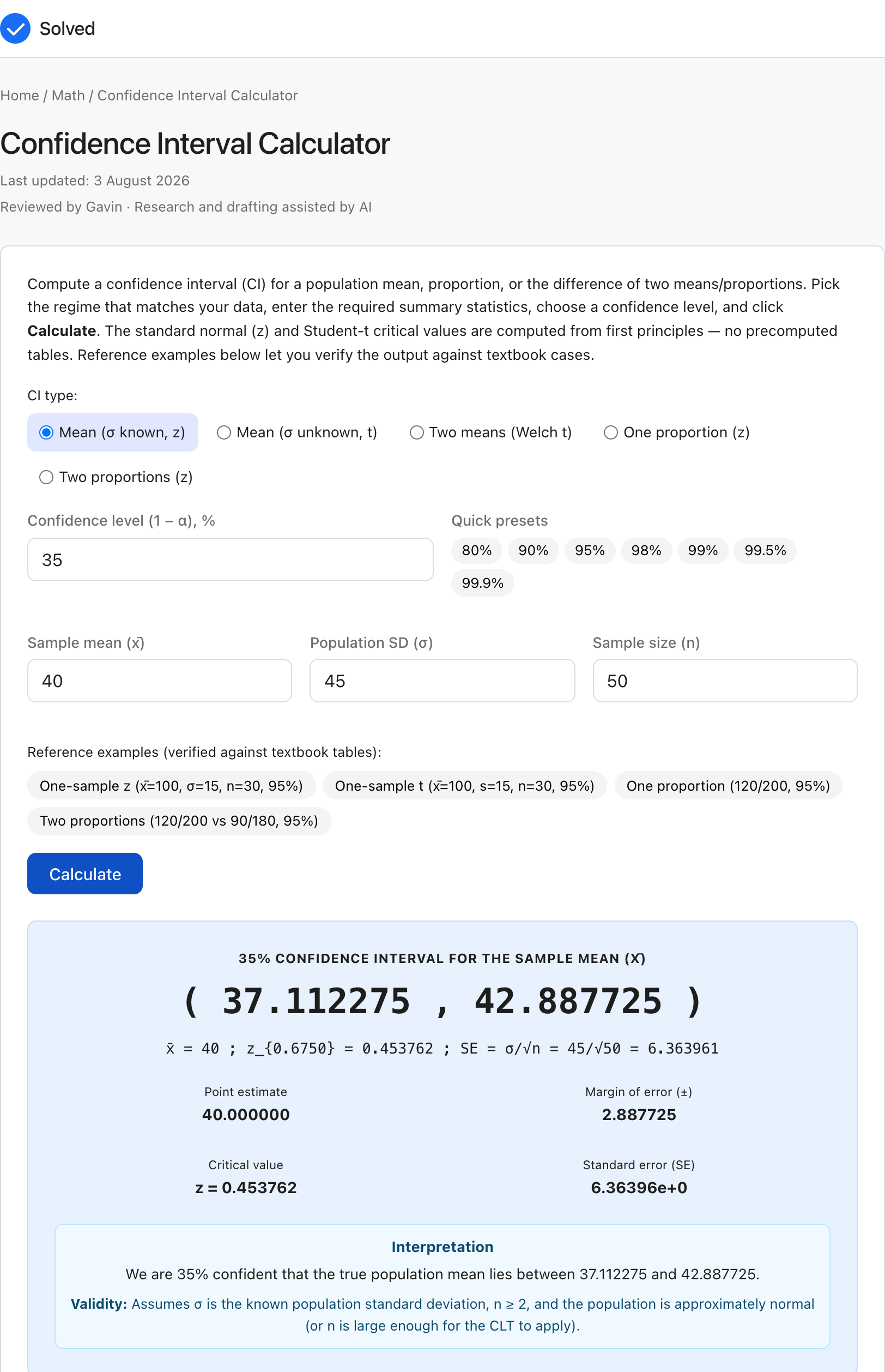
Captured from solved.tools on 10 September 2026.
Frequently Asked Questions
What is the difference between a 95% confidence interval and a 95% prediction interval? A confidence interval estimates an unknown population parameter (like the mean); a prediction interval estimates where a single future observation will fall. A 95% PI for a future observation is always wider than a 95% CI for the mean, because the future observation has both the uncertainty in the mean and the residual individual variability. Use the CI when you want to communicate where the parameter plausibly is; use the PI when you want to bracket a single new observation.
Why does the t-distribution give a wider interval than the z-distribution? When σ is unknown and is estimated from the sample, that extra uncertainty must be reflected in the interval. The t critical value tα/2, ν is always larger than zα/2 (especially for small ν), so the t-interval is wider. As the sample size grows, tα/2, ν approaches zα/2, and the two intervals converge. For n = 30, the difference is small (about 4% wider); for n = 5, it is large (about 60% wider).
Should I use a 95%, 99%, or 99.9% confidence level? The choice is a trade-off between precision and certainty. 95% is the most common default in scientific research; it leaves 5% of the long-run intervals missing the true parameter. 99% is used when a false conclusion is more costly (e.g., pharmaceutical efficacy). 90% is used in pilot or exploratory work when the cost of a false negative is low. Higher confidence → wider intervals → less precise estimates.
What does it mean when the interval includes zero (for a difference)? When the CI on a difference of means or proportions includes zero, the data are consistent with the two groups being equal at the chosen confidence level. This is the interval-estimate equivalent of a non-significant p-value. The interval communicates more than the p-value, though: a CI of (−0.5, 0.1) and a CI of (−50, 50) both include zero, but they tell very different stories about the precision of the estimate.
When should I use the Welch t-interval instead of the pooled-variance t-interval? Always, when you have two independent samples. The pooled-variance t-interval assumes the two populations have the same variance, an assumption that is rarely verified in practice and is sensitive to outliers. The Welch t-interval (this calculator's default) does not require equal variances and uses the Welch-Satterthwaite degrees of freedom to give accurate coverage even when the variances differ. Modern textbooks (and most statistical software) default to Welch for exactly this reason.
Why does the proportion CI use a normal approximation instead of an exact binomial CI? The Wald (normal-approximation) CI is the simplest closed-form CI for a proportion and is exact as n → ∞. For small n or p̂ near 0 or 1, it can extend outside [0, 1] and has poor coverage; the "exact" Clopper-Pearson CI is more accurate but is harder to invert and behaves poorly as a CI in the coverage sense. Modern recommendations (Agresti-Coull, Wilson score) are better-behaved; this calculator reports the Wald CI because it is the textbook standard and the most widely taught.
How does sample size affect the width of the confidence interval? The width of a CI is inversely proportional to √n. To halve the width of a CI, you need to quadruple the sample size. This is why small studies produce wide, uninformative intervals and why the cost of high-quality data scales as the square of the precision you need.
What if my data are not approximately normal? The mean and proportion CIs rely on either an explicit normality assumption (one-sample mean) or the central limit theorem (n large enough for the sample mean or proportion to be approximately normal). For heavily skewed data, the bootstrap CI or a conversion-based CI is more reliable. The one-sample t-interval is moderately reliable to non-normality for n ≥ 30, but for heavily skewed or heavy-tailed data, consider a non-parametric alternative.
References
- NIST/SEMATECH e-Handbook of Statistical Methods, Confidence Intervals. https://www.itl.nist.gov/div898/handbook/eda/section3/eda352.htm
- Altman, D. G., Machin, D., Bryant, T. & Gardner, M. (2013), Statistics with Confidence, 2nd ed., BMJ Books, for confidence intervals for proportions and means.