Sample Size Calculator
Last updated: 3 August 2026
Reviewed by Gavin Meiring, Lead research and primary author · Doctoral Candidate (Corporate Governance) · Research and drafting assisted by AI
Solve for the required sample size n in five common study-design scenarios — estimating a mean (z or t), a proportion, the difference of two means, or the difference of two proportions. For the one-sample cases, you specify a desired margin of error and a confidence level; the tool returns the smallest integer n that achieves the requested precision. For the two-sample cases, you additionally specify a target statistical power to detect a given effect size.
- The science of sample sizes and statistical power was formalised by Jacob Cohen, whose 1962 paper and 1969 book 'Statistical Power Analysis for the Behavioral Sciences' gave researchers their standard tables.
- The concept of power — the probability of detecting an effect that really exists — was developed by Jerzy Neyman and Egon Pearson in their landmark hypothesis-testing papers of the late 1920s and early 1930s.
- The convention of a 5% significance level traces to Ronald Fisher's 1925 'Statistical Methods for Research Workers', which spread the idea that results with p < 0.05 were worth publishing.
Sample Size Calculator
The sample size calculator solves the inverse of the confidence-interval problem: given a target precision (margin of error) or a target statistical power to detect a given effect size, what is the smallest integer n (per group, where applicable) that meets the requirement? The calculator covers five common study-design scenarios, a one-sample mean with σ known (z), a one-sample mean with σ unknown (iterative t), a one-sample proportion (Wald z), a two-sample mean with equal n per group (z, equal-variance assumption), and a two-sample proportion with equal n per group (z). Standard normal and Student-t quantiles are computed from first principles (Acklam's algorithm and bisection on the t-CDF), so the result is reproducible and exact to the limits of double-precision arithmetic.
How to Use the Sample Size Calculator
- Pick a regime using the radio buttons at the top. The five options cover the most common study-design scenarios.
- one-sample proportion), enter the design parameters: a desired margin of error and (for the unknown-σ mean) a prior estimate of s.
- two-sample proportion), enter an effect size, a common SD or two proportions, and a target power.
- Set the confidence level (1 − α), or click a preset chip for 80%, 90%, 95%, 98%, or 99%.
- also set the statistical power (1 − β), or click a preset chip for 70%, 80%, 85%, 90%, or 95%.
- Click Calculate. The result shows the required n (per group where applicable), the exact n (continuous), the formula used, and a one-sentence interpretation in plain English.
- For a quick start, click any of the reference-example chips to load a verified textbook case.
The Five Formulas
| Regime | Formula | Notes |
|---|---|---|
| Mean (σ known) | n = ( zα/2 · σ / MOE )² | Round up to integer |
| Mean (σ unknown) | Iterate from z-based n upward | tα/2, n−1 depends on n |
| Proportion | n = ( zα/2 / MOE )² · p̂ (1 − p̂) | p̂ = 0.5 gives largest n |
| Two means (equal n, equal σ) | n = 2 ( zα/2 + zβ )² σ² / δ² | Per group |
| Two proportions (equal n) | n = ( zα/2 √(2 p̄ (1−p̄)) + zβ √(p₁(1−p₁) + p₂(1−p₂)) )² / (p₁ − p₂)² | p̄ = (p₁ + p₂) / 2; per group |
In every case, the reported n is the smallest integer greater than or equal to the closed-form value (the ceiling). Rounding up rather than down is conservative, it slightly over-powers the study rather than slightly under-powering it.
Worked Example, Mean, σ Known
A quality engineer wants to estimate the mean diameter of ball bearings to within ±5 mm at the 95% confidence level. Historical data give a known population standard deviation of σ = 15 mm. How many bearings should be measured?
The critical value is z0.025 = 1.95996. The closed-form n is
n = (zα/2 · σ / MOE)² = (1.95996 × 15 / 5)² = (5.8799)² = 34.573
Rounded up, n = 35. So the engineer should measure 35 bearings to estimate the mean diameter to within ±5 mm at the 95% confidence level.
Worked Example, Proportion (Most Conservative)
A polling firm wants to estimate a candidate's vote share to within ±5 percentage points at the 95% confidence level. They have no prior estimate of the candidate's support. How many voters should be surveyed?
The most conservative choice is p̂ = 0.5, which maximises p̂ (1 − p̂) = 0.25. The closed-form n is
n = (z0.025 / MOE)² · p̂ (1 − p̂) = (1.95996 / 0.05)² × 0.25 = (39.199)² × 0.25 = 384.16
Rounded up, n = 385. So the polling firm should survey 385 voters to estimate the vote share to within ±5 percentage points at the 95% confidence level, even with no prior on p̂.
Worked Example, Proportion (With Prior)
The same polling firm has a prior estimate of p̂ = 0.3 (the candidate polls at 30% in early surveys). The closed-form n is
n = (z0.025 / MOE)² · p̂ (1 − p̂) = (1.95996 / 0.05)² × 0.3 × 0.7 = (39.199)² × 0.21 = 322.7
Rounded up, n = 323. Using a prior estimate cuts the required sample size by 16% (from 385 to 323). This is the trade-off: a good prior saves resources, but if the prior is wrong, the achieved margin of error will be wider than planned.
Worked Example, Two-Sample Mean (Effect & Power)
A clinical trial is designed to detect a 5 mmHg difference in systolic blood pressure between a new drug and a control, with 80% power at the 5% two-sided significance level. Published studies report a common SD of σ = 15 mmHg. How many patients per group are needed?
The critical values are zα/2 = 1.95996 and zβ = 0.84162 (the standard 80% power). The closed-form n per group is
n = 2 (zα/2 + zβ)² σ² / δ² = 2 × (1.95996 + 0.84162)² × 225 / 25 = 2 × 7.8478 × 9 = 141.26
Rounded up, n = 142 per group, for a total enrolment of 284 patients.
Worked Example, Two-Sample Proportion (Effect & Power)
A product team is running an A/B test to detect a 2 percentage-point uplift in conversion rate (8% → 10%), with 80% power at the 5% two-sided significance level. How many users per group are needed?
The critical values are zα/2 = 1.95996 and zβ = 0.84162. The pooled proportion is p̄ = 0.09. The closed-form n per group is
n = (zα/2 √(2 p̄ (1−p̄)) + zβ √(p₁(1−p₁) + p₂(1−p₂)))² / (p₁ − p₂)² = (1.95996 × √(0.1638) + 0.84162 × √(0.0736 + 0.0900))² / 0.0004 = (1.95996 × 0.4047 + 0.84162 × 0.4045)² / 0.0004 = (0.7932 + 0.3404)² / 0.0004 = (1.1336)² / 0.0004 = 1.2850 / 0.0004 = 3212.6
Rounded up, n = 3,213 per group, for a total of 6,426 users. This is a much larger experiment than the proportion-with-prior case above because the effect size is small (2 percentage points on a baseline of 8%).
What Is Statistical Power?
Statistical power is the long-run probability that a study of size n will reject the null hypothesis at level α when a true effect of size δ exists. Power 1 − β is set by convention: 80% is the most common default in scientific research, 90% in clinical trials and pharmaceutical work, 95% in confirmatory settings. The relationship between n, power, and effect size is approximately n ∝ (zα/2 + zβ)² σ² / δ². Doubling the power (e.g. 80% → 95%) requires roughly 1.7× the n, not 2×. Halving the effect size to detect requires 4× the n. This is why pilot studies of small effects are so expensive, and why the choice of δ is the most consequential design decision.
Why the Answer Is Always an Integer
Sample size is a count of observations and must be a positive integer. The closed-form nExact is a real number; the calculator reports the smallest integer ≥ nExact (the ceiling). This is conservative: rounding down to the nearest integer would slightly underpower the study. two-sample cases, the same ceiling rule applies independently to the n-per-group figure; the total sample size is 2 × ceiling(n).
Common Pitfalls
Using the z-based mean formula when σ is unknown. If the sample SD is the only available estimate of variability, the t-based n is what you need, it is slightly larger than the z-based n (a few percent for n ≥ 30, much more for n < 15). The calculator handles the iteration automatically.
Using p̂ = 0.5 when you have a better estimate. p̂ = 0.5 gives the most conservative (largest) n, but if you know p̂ is around 0.1 or 0.9, the true n is much smaller. A 50% reduction in p̂(1 − p̂) roughly halves the n required.
Confusing n with the total sample size. two-sample cases, the reported n is per group. The total sample size is 2 × n. A study with n = 142 per group is a 284-participant study, not a 142-participant study.
Forgetting the normal-approximation validity condition for proportions. The proportion-based formulas assume n·p̂ ≥ 10 and n·(1−p̂) ≥ 10. For p̂ near 0 or 1, or n small, the actual required n may be larger than the formula suggests.
Underestimating σ. For a continuous outcome, an underestimated σ leads to an underestimated n and an underpowered study. Pilot data, published similar studies, and the rule of thumb "σ is about ¼ to ½ of the plausible range" are all common sources for a prior σ.
Finite Population Correction
If your sample is a non-negligible fraction of a finite population of size N, the required n is reduced by the finite population correction (FPC): nadj = n / (1 + n / N). For n << N, the correction is tiny (and the calculator ignores it); for n approaching N, the reduction can be substantial. The FPC is not exposed in the current UI but the formula is straightforward to apply to the reported n.
How the Calculator Computes the Quantiles
Standard normal quantiles are computed with Peter Acklam's algorithm (an inverse-CDF approximation accurate to about 10⁻⁹ over the entire real line). Student-t quantiles for the iterative mean-t case are computed by bisection on the t-CDF, where the t-CDF itself is built from the regularized lower incomplete beta function Ix(a, b) via a continued-fraction routine (Numerical Recipes style, Lentz's method). The two-sample formulas use only the standard normal quantile (zα/2 and zβ).
Real-World Applications
Sample-size calculations appear in every quantitative discipline that designs experiments or surveys. In polling and survey research, a polling firm deciding how many voters to call to estimate a proportion to within ±3% at the 95% confidence level uses the one-proportion formula with p̂ = 0.5. In clinical trials, a trial designed to detect a 5 mmHg difference in systolic blood pressure between treatment and control at 80% power uses the two-sample mean formula. In A/B testing, a product team deciding how many users to enrol in a conversion-rate test to detect a 2 percentage-point uplift uses the two-sample proportion formula. In quality control, a manufacturing process that needs a CI on the mean within a tight tolerance to confirm a specification uses the one-sample mean formula. In ecological and environmental surveys, a survey designed to estimate a species' abundance to within ±10% of the true value uses the one-sample mean (or proportion) formula with σ estimated from prior surveys.
Reference Table: Sample size by margin of error and confidence
Required responses for a proportion survey, assuming the most conservative case of a 50% result and an infinite population. A 5% margin at 95% confidence needs 385 responses; halving the margin to 2.5% roughly quadruples the requirement.
| Margin of error | Confidence | z value | Responses needed |
|---|---|---|---|
| 2% | 90% | 1.645 | 1,692 |
| 2% | 95% | 1.96 | 2,401 |
| 2% | 99% | 2.576 | 4,148 |
| 3% | 90% | 1.645 | 752 |
| 3% | 95% | 1.96 | 1,068 |
| 3% | 99% | 2.576 | 1,844 |
| 5% | 90% | 1.645 | 271 |
| 5% | 95% | 1.96 | 385 |
| 5% | 99% | 2.576 | 664 |
Worked Example on Screen
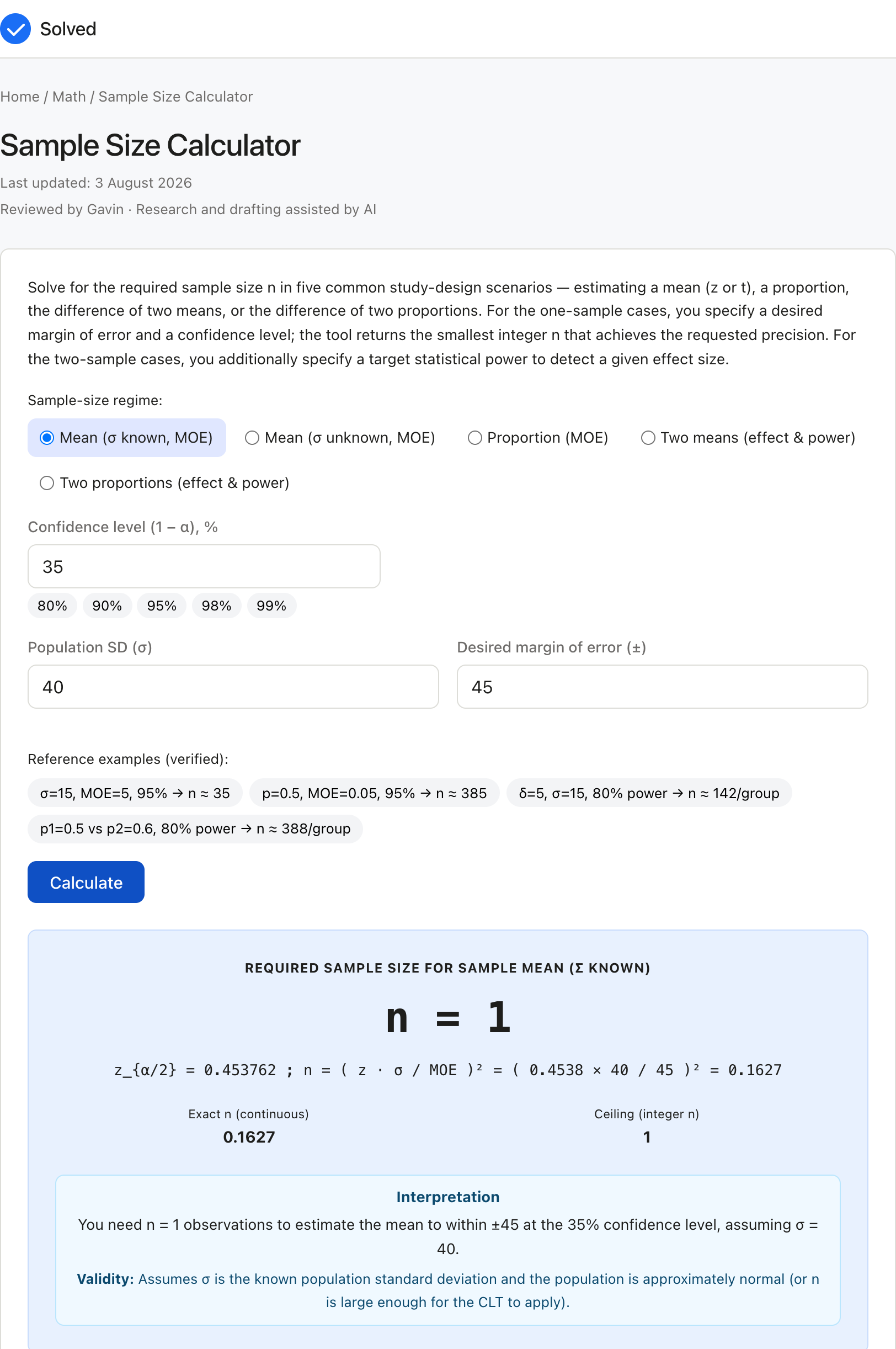
The capture below shows Sample Size Calculator after the inputs were entered, with the result on screen. Enter the same values to reproduce it.
Captured from solved.tools on 10 September 2026.
Frequently Asked Questions
What's the difference between "n for a margin of error" and "n for a given power"? They are different design questions. The margin-of-error case asks: "How many observations do I need to estimate a parameter to a given precision?" The power case asks: "How many observations per group do I need to detect a given effect size with a given probability?" The first is appropriate for descriptive studies; the second for comparative studies. The formulas are different (the power case has both zα/2 and zβ; the MOE case has only zα/2), and the required n is typically much smaller in the MOE case for the same confidence level.
What power should I use? 80% is the conventional default in most scientific research; 90% in clinical trials and pharmaceutical work; 95% in confirmatory settings. The choice is a trade-off between study cost and the cost of missing a true effect. Higher power requires more participants (and higher cost) but reduces the false-negative rate. The relationship is roughly that doubling the power from 80% to ~95% requires 1.7× the n, not 2×.
What if my prior estimate of σ is wrong? A wrong prior σ leads to a wrong n. An underestimated σ produces an underpowered study (lower actual power than planned); an overestimated σ produces an over-powered study (wasted resources). The conservative move is to use a slightly larger σ than you think is right, or to do a small pilot study to refine the estimate. The rule of thumb "σ is about ¼ to ½ of the plausible range of the outcome" is one common approach when no prior is available.
Should I use a one-tailed or two-tailed test for the power calculation? The calculator uses a two-sided test (zα/2) by default, which is the standard in most applications. For a one-sided test, replace zα/2 with zα in the formula, the required n is slightly smaller. One-sided tests are appropriate when the direction of the effect is known a priori (e.g. "the new drug is at least as good as the old one"). Two-sided tests are appropriate when the direction is uncertain.
How does the equal-variance assumption affect the two-sample mean n? The closed-form two-sample mean formula n = 2 (zα/2 + zβ)² σ² / δ² assumes equal variances in the two groups. If the variances are very different, the required n is asymmetric (the group with the larger variance needs more participants), and a Welch-t formulation is more appropriate. The calculator exposes only the equal-variance case; for unequal variances, a different (iterative) formula is required.
What's a good rule of thumb for the proportion case? For a 95% confidence level and ±5% margin of error with no prior on p̂, the most conservative n is 385 (using p̂ = 0.5). For ±3% it's about 1068; for ±1% it's about 9604. If you know p̂ is around 0.1, the same ±5% requires only 138; if p̂ is around 0.3, it requires about 323. Knowing the approximate p̂ can dramatically reduce the required n.
Why is the answer an integer and not the formula's exact value? Sample size is a count of observations and must be a positive integer. The closed-form nExact is a real number; the calculator reports the smallest integer ≥ nExact (the ceiling). Rounding up rather than down is conservative, it slightly over-powers the study rather than slightly under-powering it. The exact value is also reported so the user can see how close the ceiling is to the continuous value.
What if I need unequal n per group (e.g. 2:1 allocation)? The closed-form formula assumes equal allocation. For a 2:1 allocation (twice as many in one group as the other), the total sample size is about 12% larger than the equal-allocation case for the same power. The exact formula is n1 = (1 + 1/k)² · (zα/2 + zβ)² σ² / δ² and n2 = n1 / k, where k is the allocation ratio. The calculator does not expose this case but the extension is straightforward.
References
- NIST/SEMATECH e-Handbook of Statistical Methods, Sample Size Determination. https://www.itl.nist.gov/div898/handbook/prc/section2/prc222.htm
- Cochran, W. G. (1977), Sampling Techniques, 3rd ed., Wiley, for the standard formulas for sample size under simple random sampling.